Markov's inequality
In probability theory, Markov's inequality gives an upper bound for the probability that a non-negative function of a random variable is greater than or equal to some positive constant. It is named after the Russian mathematician Andrey Markov, although it appeared earlier in the work of Pafnuty Chebyshev (Markov's teacher), and many sources, especially in analysis, refer to it as Chebyshev's inequality or Bienaymé's inequality.
Markov's inequality (and other similar inequalities) relate probabilities to expectations, and provide (frequently) loose but still useful bounds for the cumulative distribution function of a random variable.
An example of an application of Markov's inequality is the fact that (assuming incomes are non-negative) no more than 1/5 of the population can have more than 5 times the average income.
Contents |
Statement
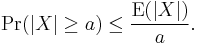
If X is any random variable and a > 0, then
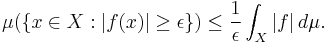
In the language of measure theory, Markov's inequality states that if (X, Σ, μ) is a measure space, ƒ is a measurable extended real-valued function, and  , then
Corollary: Chebyshev's inequality
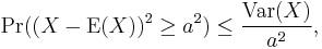
Chebyshev's inequality uses the variance to bound the probability that a random variable deviates far from the mean. Specifically:
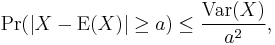
for any a>0. Here Var(X) is the variance of X, defined as:
![\operatorname{Var}(X) = \operatorname{E}[(X - \operatorname{E}(X) )^2].](/2012-wikipedia_en_all_nopic_01_2012/I/569f5010da4d87d4dc3f5c4a910f8cb7.png)
Chebyshev's inequality follows from Markov's inequality by considering the random variable
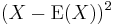
for which Markov's inequality reads
Proofs
We separate the case in which the measure space is a probability space from the more general case because the probability case is more accessible for the general reader.
In the language of probability theory
For any event E, let IE be the indicator random variable of E, that is, IE = 1 if E occurs and = 0 otherwise. Thus I(|X| ≥ a) = 1 if the event |X| ≥ a occurs, and I(|X| ≥ a) = 0 if |X| < a. Then, given a > 0,
which is clear if we consider the two possible values of I(|X| ≥ a). Either |X| < a and thus I(|X| ≥ a) = 0, or I(|X| ≥ a) = 1 and by the condition of I(|X| ≥ a), the inequality must be true.
Therefore
Now, using linearity of expectations, the left side of this inequality is the same as
Thus we have
and since a > 0, we can divide both sides by a.
In the language of measure theory
We may assume that the function  is non-negative, since only its absolute value enters in the equation. Now, consider the real-valued function s on X given by
Then  is a simple function such that
  . By the definition of the Lebesgue integral

and since , both sides can be divided by  , obtaining
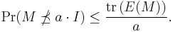
Matrix-valued Markov
Let  be a self adjoint matrix-valued random variable and
  . Then
Examples
- Markov's inequality is used to prove Chebyshev's inequality.